How to calculate a Pokemons 'power level' using kmeans

Table of Contents

• The Heros Journey
• Grouping and counting
• evolves_from_species
• TM01 (e.g. Tidy Models 01)
  • How kmeans works
  • How to use it
• Conclusion

library(pokedex)
library(tidyverse)
library(tidymodels)
library(showtext)
font_add_google("Press Start 2P")
showtext_auto()

theme_set(theme_pokedex())

knitr::opts_chunk$set(fig.showtext=TRUE)

The Heros Journey

Pokemon games have a very familiar cycle. You start with one of 3 Pokemon. You adventure out with your new buddy, facing tougher and tougher Pokemon, in greater variety. Many of your Pokemon evolve over time, and eventually you find the end-game legendaries in a climactic battle of titans!

You can even see this story in the data. Here is the base_experience of all the Pokemon, identified by game generation. The base_experience is the basic amount of experience that is gained by the winner of a battle from a specific species. e.g. If you beat a Bulbasaur, your Pokemon gains experience based on a formula which uses Bulbasaurs base_experience. Because of that we can see it as a proxy value for how powerful a Pokemon is. If it’s more powerful, it will be harder to beat, and so reward you with more experience when you win.

pokemon %>%
  ggplot(aes(x = id, y = base_experience, colour = generation_id)) +
  geom_point() +
  labs(title = "Base Experience for each Pokemon")

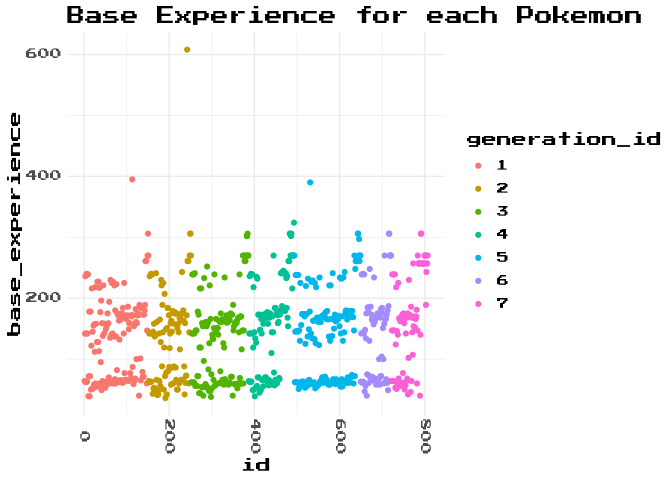
In each generation you can see a few attributes:

• power level - 3(ish) tiers, grouped in different vertical lanes
• progression - a (generally) increasing trend in the base power value
• the up-ticks at the start and the end of each gen are the starters top-tier evolution (Woo Blastoise!) and the Legendaries at the end-game

Lets see if we can group each Pokemon into a power_level. A categorical grouping which relates it to other Pokemon with similar base_experience

Grouping and counting

Maybe we can explicitly describe the power levels of each tier of Pokemon with a simple process? Can we group each Pokemon by evolutionary chain, and then count each Pokemons order within the group?

pokemon %>%
  group_by(evolution_chain_id) %>%
  mutate(power_level = row_number()) -> pokemon_group_count

ggplot(pokemon_group_count,
       aes(
    x = id,
    y = base_experience,
    colour = as_factor(power_level)
  )) +
  geom_point() +
  labs(title = "Power level by group count",
       colour = "power_level")

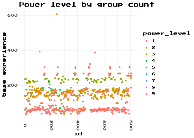
Sort of? Generally we capture the pattern, but we don’t actually get it very right. First off, there are more than 3 evolutionary tiers in our engineered feature. We can also see there are some Pokemon are classified as a power_level higher than 1, but still in the lowest group on this list. Why might have caused this?

pokemon_group_count %>%
  filter(power_level > 3) %>%
  pull(evolution_chain_id) -> pokemon_group_count_mistakes

pokemon_group_count %>%
  filter(evolution_chain_id %in% pokemon_group_count_mistakes) %>%
  select(id,
         name,
         base_experience,
         generation_id,
         evolution_chain_id,
         power_level)  %>%
  arrange(evolution_chain_id) %>%
  select(id, name, base_experience, evolution_chain_id, power_level) %>% 
  knitr::kable()

So there are some clear problems with this approach. In Gen 1 we had some branching evolution with the Eevee family. Not only was this family expanded in multiple generations to eventually 8 variations, but we also saw more branching evolution trees as well. We also got ‘baby’ Pokemon. Pokemon that are actually pre-cursors to other Pokemon, but are listed later in the Pokedex.

Luckily there is another variable we can use, that should be a whole lot better.

evolves_from_species

Each Pokemon that evolves from another Pokemon has the Pokemon they evolve froms id as the value in the evolves_from_species_id variable. Maybe we can use that to break up the Pokemon into their ‘power levels’.

The following code is not my best work, however I spent some time on a more recursive strategy, but it was honestly miles more confusing. For the purposes of a silly example for a blog, I think this is prefferable.

pokemon %>%
  mutate(power_level = case_when(is.na(evolves_from_species_id) ~ 1)) %>%
  filter(power_level == 1) -> pokemon_1

pokemon %>%
  mutate(power_level = case_when(evolves_from_species_id %in% pokemon_1$id ~ 2)) %>%
  filter(power_level == 2) -> pokemon_2

pokemon %>%
  mutate(power_level = case_when(evolves_from_species_id %in% pokemon_2$id ~ 3)) %>%
  filter(power_level == 3) -> pokemon_3

bind_rows(pokemon_1, pokemon_2, pokemon_3) %>%
  arrange(id) %>%
  mutate(power_level = as_factor(power_level)) -> pokemon_evolves_from

pokemon_evolves_from %>%
  ggplot(aes(x = id, y = base_experience, colour = power_level)) + 
  geom_point() +
  labs(title = "Power level by evolves_from")

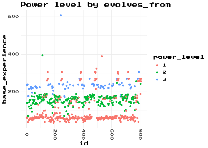
Hmm, that’s actually worse? Lets focus on the Pokemon labelled power_level 1, but are up where we would expect level 3 Pokemon to be.

pokemon_evolves_from %>% 
  filter(base_experience > 200 & power_level == 1) %>% 
  select(id, name, base_experience) %>% 
  knitr::kable()

So these Pokemon are nearly all ‘Legendary’. They are big end-game Pokemon, with real rarity in game. They also don’t evolve from, or to, anything, so our rule doesn’t classify them effectively.

pokemon_evolves_from %>% 
  filter(base_experience < 200 & base_experience > 100 & power_level == 1) %>% 
  select(id, name, base_experience) %>% 
  knitr::kable()

These Pokemon are not end game, but they either have very short evolution trees (2 Pokemon long), or no evolution tree at all.

So our ‘group count’ process doesn’t work well, and neither does our ‘evolves_from_species’ process. We’re going to have to to learn some new moves.

TM01 (e.g. Tidy Models 01)

Clustering is the process of using machine learning to derive a categorical variable from data. The simplest form of clustering that seems relevant to our problem is k-means. Seeing as we have a pretty good intuition that 3 groups implicitly exist in this data, and a clear visualisation supporting us, lets cut straight to asking R for 3 groups. k-means clustering aims to divide the data into a known number of groups which is set in the centers argument, and doesn’t require any data to be fed to it as examples of what makes up a ‘group’. That sentence might be a little confusing, as we do obviously give it some data. What we don’t give it is a training data set which has examples of what Pokemon are supposed to be in a given group, labelled with the group they are supposed to be in, e.g. Squirtle is in group 1, Wartortle is in group 2, Blastoise is in group 3, and then give it unlabelled data to classify, e.g. “What group is Charmeleon in?”. k-means will figure out how to split the continuous variable base_experience into 3 groups.

set.seed(68)

pokemon %>% 
  select(base_experience)  %>% 
  kmeans(centers = 3) %>% 
  augment(pokemon) -> pokemon_cluster

How kmeans works

First, we set centroids to be at random positions in the data. To make sure this doesn’t effect consistency in my article I’ve used set.seed so k-means starts looking for the centres of our clusters from the same position each time. A ‘centroid’ can be seen as a ‘centre point’ for each cluster. We have the same number of centroids set as the value set in the centers argument. Each data point is then assigned to it’s closest centroid.

The Sum of Squared Errors (SSE) from the centroids is then used as an objective function towards a local minimum.

This is the core concept of how k-means calculates a solution. The Sum of Squared Errors are calculated like this:

{% katex %} \sum^n_{i-1}(x_i-\bar{x})^2 {% endkatex %}

What this means is for each group, the distance from the centroid to each observation is measured, and then squared. Then each of those squared distances, one per observation in the group, is totalled.

The centroid is then moved to the average value of it’s group. Because the centroids are now no longer in the same position as when the SSE was calculated, the SSE is now recalculated for all observations, to each of the new centroid positions. This means that some observations are now closer to a different centroid, and so get assigned to a different cluster.

Then the centroids are moved again to the new average of the new cluster. Each cluster then gets new distances calculated. This will go on until termination when, each centroid is in the average position of the cluster, and each observation in the cluster is closest to the centroid it is currently assigned to.

That’s a slightly wordy description of a complicated process. I recommend that you have a look at the k-means explanation in tidy models to really cement the concept. It also contains the most adorable animation of a statistical concept in existance.

How to use it

Here, I’ve simply selected the one column of data, base_experience, and piped it into kmeans, which is part of base R. This returns a super un-tidy list like object of class "kmeans", however, with tidymodels we can easily make it usable.

augment helps us to match the output of the kmeans function back to our data for easier processing. The output of kmeans doesn’t actually contain any of the other information about our data, it only got given one column remember? augment goes through the return of kmeans, finds the relevant bit, and matches it neatly back to our original data ready for plotting in one step!

pokemon_cluster %>% 
  ggplot(aes(x = id, y = base_experience, colour = .cluster)) +
  geom_point() +
  labs(title = "Power level by kmeans clustering")

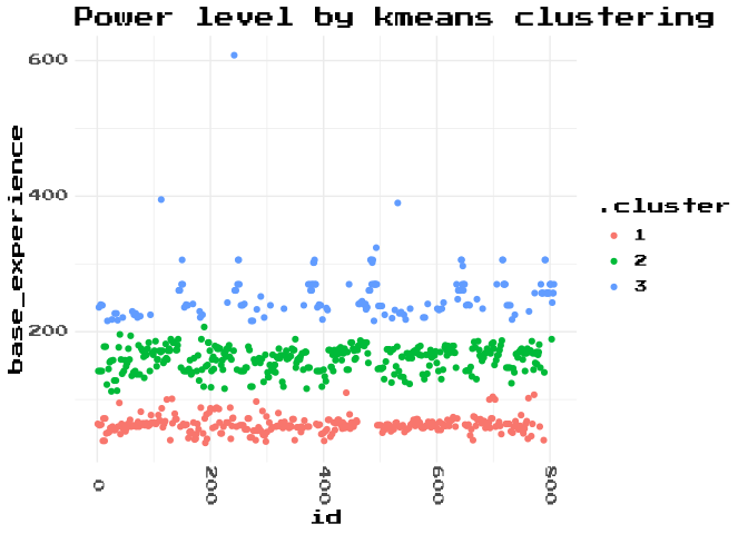
This is a lot better. It gives us really clear groups, in exactly where we expected them. It’s also tonnes simpler code!

Lets check some of our boundary positions, just to make sure it makes sense.

pokemon_cluster %>% 
  filter(.cluster == 1 & base_experience > 100) %>% 
  select(id, name, base_experience) %>% 
  knitr::kable()

pokemon_cluster %>% 
  filter(.cluster == 2 & base_experience > 200) %>% 
  select(id, name, base_experience) %>% 
  knitr::kable()

Ditto and Type: Null are just a plain weird Pokemon due to their abilities messing with their type. Happiny is a baby type, but from a family with an insane base_experience. Jumpluff is an awkward edge case. Technically the 3rd evolution, it’s still got an extremely low base_experience. Potentially this is for game balancing as they are relatively regularly encountered? Aurorus and Steenee I do not have a good hypothesis for.

Generally I think that this is a pretty good solution. There are maybe a few edge cases that are open to interpretation, but that’s just what we get sometimes with machine learning. Lacking a labelled training data set, we can’t compute a confusion matrix or ROC-curve.

Conclusion

We’ve found a situation in the ‘real’ world where we know from context there is a categorical relationship, but from the data available it’s not possible to classify that precisely. However we can create this categorisation using machine learning! Even better, we can use the tidymodels package to help us do it quickly and cleanly.

Go to top

Read Next

Read Previous